Recurrent neural networks are very famous deep learning networks which are applied to sequence data: time series forecasting, speech recognition, sentiment classification, machine translation, Named Entity Recognition, etc..
The use of feedforward neural networks on sequence data raises two majors problems:

• Input & outputs can have different lengths in different examples
• MLPs do not share features learned across different positions of the data sample

In this article, we will discover the mathematics behind the success of RNNs as well as some special types of cells such as LSTMs and GRUs. We will finally dig into the encoder-decoder architectures combined with attention mechanisms.

NB: Since Medium does not support LaTeX, the mathematical expressions are inserted as images. Hence, I advise you to turn the dark mode off for a better reading experience.

The summary is as follows:

1. Notation
2. RNN model
3. Different types of RNNs
4. Advanced types of cells
5. Encoder & Decoder architecture
6. Attention mechanisms

‍

Notation

As an illustration, we will consider the task of Named Entity Recognition which consists of locating and identifying the named entity such as proper names:

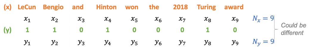
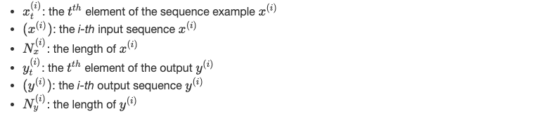
We denote:

When dealing with non-numerical data, text, for instance, it is very important to encode it to numerical vectors: this operation is called embedding. One of the most famous ways to encode text is Bert which was developed by Google.

RNN model

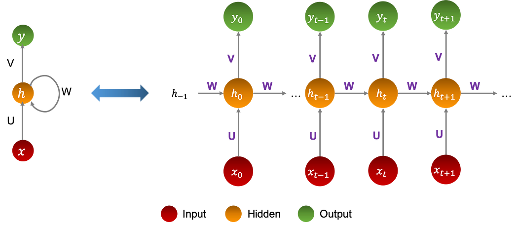
RNNs represent a special case of neural networks where the parameters of the model, as well as the operations performed, are the same throughout the architecture. The network performs the same task for each element in a sequence whose output depends on the input and the previous state of the memory.
The graph below shows a neural network of neurons having a single layer of hidden memory:

Equations

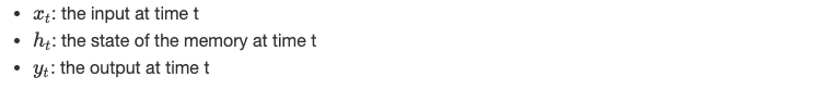
The variables in the architecture are:

where:

h(−1)​ is randomly initialized, ϕ and ψ are non-linear functions, U, V, and W are parameters of the various linear regressions, preceding the nonlinear activations.
It is important to note that they are the same throughout the architecture.

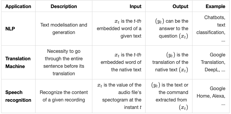
Applications

Recurrent neural networks have significantly improved sequential models, in particular :

• NLP Tasks, Modeling and Text Generation
• Translation machine
• Voice recognition

We summarize the above applications in the following table:

Learning algorithm

As in classical neural networks, learning in the case of recurrent networks is done by optimizing a cost function with respect to U, V and W. In other words, we aim to find the best parameters that give the best prediction y^i, starting from the input xi​, of the real value yi​.

For this, we define an objective function called the loss function and denoted J which quantifies the distance between the real and the predicted values on the overall training set.

We minimize J following two major steps:

• Forward Propagation: we propagate the data through the network either in entirely or in batches, and we calculate the loss function on this batch which is nothing but the sum of the errors committed at the predicted output for the different rows.
• Backward Propagation Through Time: consists of calculating the gradients of the cost function with respect to the different parameters, then apply a descent algorithm to update them. It is called BPTT, since the gradients at each output depend both on the elements of the same instant and the state of the memory at the previous instant.

We iter the same process a number of times called epoch number. After defining the architecture, the learning algorithm is written as follows:

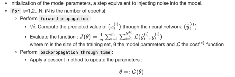
(∗) The cost function L evaluates the distances between the real and predicted value on a single point.

Forward propagation

Let us consider the prediction of the output of a single sequence through the neural network.
At each moment t, we compute:

Until reaching the end of the sequence.
Again, the parameters U, W and V remain the same all along the neural network.
When dealing with an m-row data set, repeating these operations separately for each line is very costly. Hence, we truncate the dataset in order to have sequences described in the same timeline, i.e:

We can use linear algebra to parallelize it as follows:

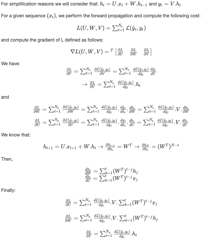
Backpropagation Through Time

The backpropagation is the second step of the learning, which consists of injecting the errorcommitted in the prediction (forward) phase into the network and update its parameters to perform better on the next iteration. Hence, the optimization of the function J, usually through a descent method.

We can now apply a descend method as detailed in my previous article.

Memory problem

There are several fields where we are interested in predicting the evolution of a time serie based on its history: music, finance, emotions…etc.
The intrinsic recurrent networks described above, called ‘Vanilla’, suffer from a weak memory unable to take into account several elements of the past in the prediction of the future.

With this in mind, various extensions of the RNNs have been designed to trim the internal memory: bi-directional neural networks, LSTM cells, attention mechanisms…etc. Memory enlargement can be crucial in certain fields such as finance where one seeks to memorize as much history as possible in order to predict a financial series.

The learning phase in RNN might also suffer from gradient vanishing or gradient exploding problems since the gradient of the cost function includes the power of W which affects its memorizing capacity.

‍

Different types of RNNs

There are several extensions for classic or ‘Vanilla’ recurrent neural networks, these extensions have been designed to increase the memory capacity of the network along with the features extraction capacity.
The illustration below summarizes the different extensions:

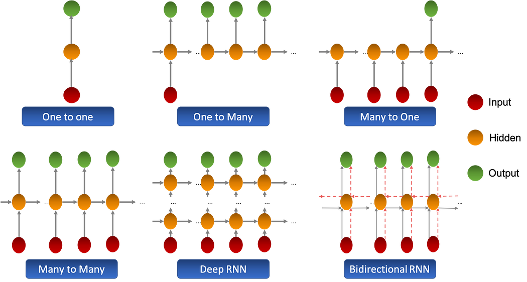
There exist other types of RNNs that have a specifically designed hidden layer which we will discuss in the next chapter.

‍

Advanced types of cells

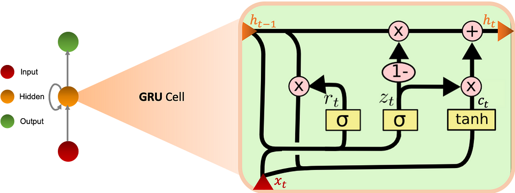
Gated Recurrent Unit

GRU (Gated Recurrent Unit) cells allow the recurrent network to save more historical information for a better prediction. It introduces an update gate which determines the quantity of information to keep from the past as well as a reset gate which sets the quantity of information to forget.
The graph bellow schematizes the GRU cell:

Equations
We define the equations in the GRU cell as follows:

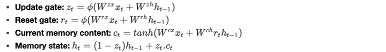
ϕ is a non-linear integer function and the parameters W are learned by the model.

Long Short Term Memory

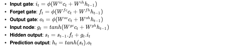
LSTMs (Long Short Term Memory) were also introduced to overcome the problem of short memory, they have 4 times more memory than Vanilla RNNs. This model uses the notion of gates and has three :

• Input gate i: controls the flow of incoming information.
• Forget gate f: Controls the amount of information from the previous memory state.
• Output gate o: controls the flow of outgoing information

The graph below shows the operation of the LSTM cell:

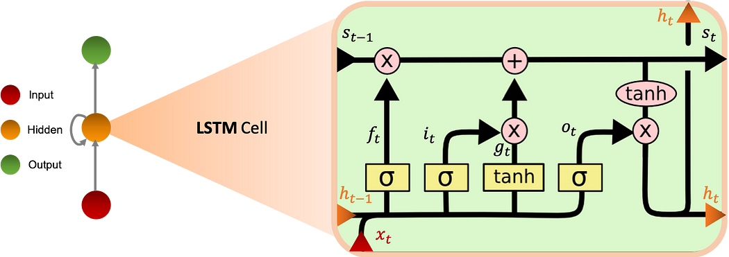
When the input and output doors are closed, activation is blocked in the memory cell.

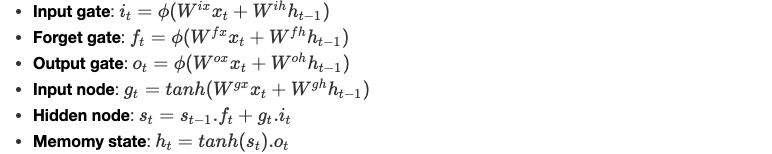
Equations
We define the equations in the LSTM cell as follows:

Pros & Cons
We can summarize the advantages and disadvantages of LSTM cells in 4 main points:

• Advantages

+They are able to model long-term sequence dependencies.
+They are more robust to the problem of short memory than ‘Vanilla’ RNNs since the definition of the internal memory is changed from:

• Disadvantages

+They increase the computing complexity compared to the RNN with the introduction of more parameters to learn.
+The memory required is higher than the one of ‘Vanilla’ RNNs due to the presence of several memory cells.

‍

Encoder & Decoder architecture

It is a sequential model consisting of two main parts:

• Encoder: the first part of the model processes the sequence and then returns at the end an encoding vector of the whole series called context vector which summarizes the information of the different inputs.
• Decoder: the context vector is then taken as the input to the decoder in order to make the predictions.

The diagram below illustrates the architecture of the model :

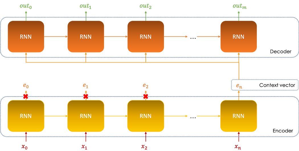
The encoder can be considered as a dimension reduction tool, matter of fact, the context vector en​ is nothing else than the encoding of the input vectors (in0​,in1​,…inn​), the sum of the sizes of these vectors is much larger than that of en, hence the notion of dimension reduction.

‍

Attention mechanisms

Attention mechanisms were introduced to address the problem of memory limitation, and mainly answer the following two questions:

• What weight (importance) αj​ is given to each output ej​ of the encoder?
• How can we overcome the limited memory of the encoder in order to be able to ‘remember’ more of the encoding process?

The mechanism inserts itself between the encoder and the decoder and helps the decoder to significantly select the encoded inputs that are important for each step of the decoding process outi​ as follows:

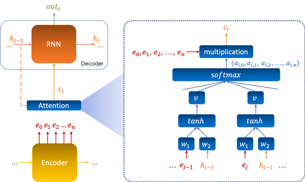
Mathematical formalism

Keeping the same notation as before, we set αi,j​ as the attention given by the output i, denoted outi​, to the vector ej​.
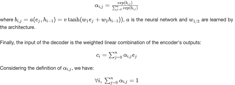
The attention is computed via a neural network which takes as inputs the vectors (e0​,e1​,…,en​) and the previous memory state h(i-1)​, it is given by:

Application: Translation Machine

The use of an attention mechanism makes it possible to visualize and interpret what the model is doing internally, especially at the time of prediction.
For example, by plotting a 'heatmap' of the attention matrix of a translation system, we can see the words in the first language on which the model focuses to translate each word into the second language:

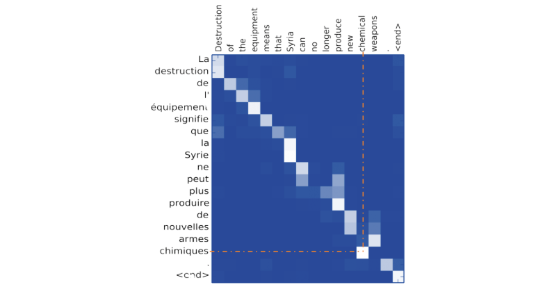
As illustrated above, when translating a word into English, the system focuses in particular on the corresponding French word.

Overlay of LSTM & Attention Mechanism

It is relevant to combine the two methods to improve internal memory, since the first one allows more elements of the past to be taken into account and the second one chooses to pay careful attention to them at the time of prediction.
The output ct of the attention mechanism is the new input of the LSTM cell, so the system of equations becomes as follows :

ϕ is a non-linear integer function and the parameters W are learned by the model.

‍

Conclusion

RNNs are a very powerful tool to deal with sequence data, they provide incredible memorizing capacities and are widely used in day-to-day life.
They also have many extensions which enable to address various types of data-driven problems, more particularly the ones discussing times series.

Do not hesitate to check my previous article dealing with:

• Deep Learning’s mathematics
• Convolutional Neural Networks’ mathematics
• Object detection & Face recognition algorithms

‍

References

• Z.Lipton, J.Berkowitz, C.Elkan, A Critical Review of Recurrent Neural Networks for Sequence Learning, arXiv: 1506.00019v4, 2015.
• H.Salehinejad, S.Sankar, J.Barfett, E.Colak, S.Valaee, Recent Advances in Recurrent Neural Networks, arXiv: 1801.01078v3, 2018.
• Y.Baveye, C.Chamaret, E.Dellandréa, L.Chen, Affective Video Content Analysis: A Multidisciplinary Insight, HAL Id: hal-01489729, 2017.
• A.Azzouni, G.Pujolle, A Long Short-Term Memory Recurrent Neural Network Framework for Network Traffic Matrix Prediction, arXiv: 1705.05690v3, 2017.
• Y.G.Cinar, H.Mirisaee, P.Goswami, E.Gaussier, A.Ait-Bachir, V.Strijov, Time Series Forecasting using RNNs: an Extended Attention Mechanism to Model Periods and Handle Missing Values, arXiv: 1703.10089v1, 2017.
• K.Xu, L.Wu, Z.Wang, Y.Feng, M.Witbrock, V.Sheinin, Graph2Seq: Graph to Sequence Learning with Attention-Based Neural Networks, arXiv: 1804.00823v3, 2018.
• Rose Yu, Yaguang Li, Cyrus Shahabi, Ugur Demiryurek, Yan Liu, Deep Learning: A Generic Approach for Extreme Condition Traffic Forecasting, Southern California university, 2017.