Deep learning is a subfield of Machine Learning Science which is based on artificial neural networks. It has several derivatives such as Multi-Layer Perceptron-MLP-, Convolutional Neural Networks -CNN- and Recurrent Neural Networks -RNN- which can be applied to many fields including Computer Vision, Natural Language Processing, Machine Translation…

Deep learning is taking off for three main reasons:

• Instinctive features engineering: while most of machine learning algorithms require human expertise for the feature engineering and extraction, deep learning handles automatically the choice of variables and their weights
• Huge Datasets: the continuous collection of data has led to large databases which allow deeper neural networks
• Hardware evolution: the new GPUs, for Graphical Process Units, allow faster algebraic calculation which is the core base of DL

In this blog, we will focus mainly on the Multi-Layer Perceptron -MLP- where we will detail the mathematical background behind the success of deep learning and explore the optimization algorithms used to improve its performances.

The summary is as follows:

1. Definition
2. Learning algorithm
3. Parameter Initialization
4. Forward — Backpropagation
5. Activation functions
6. Optimization algorithm

NB: Since Medium does not support LaTeX, the mathematical expressions are inserted as images. Hence, I advise you to turn the dark mode off for a better reading experience.

‍

Definition

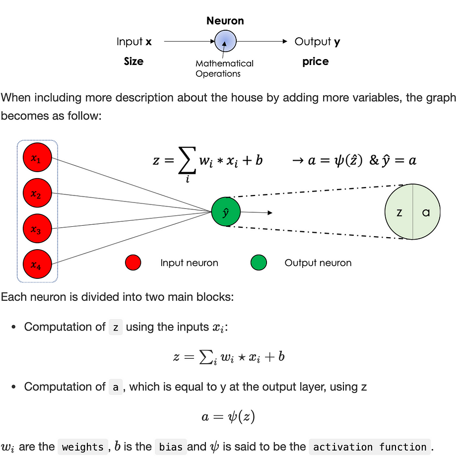
A neuron

It is a bloc of mathematical operations linking entities

Let’s consider the problem where we estimate the price of a house based on its size, it can be schematized as follows:

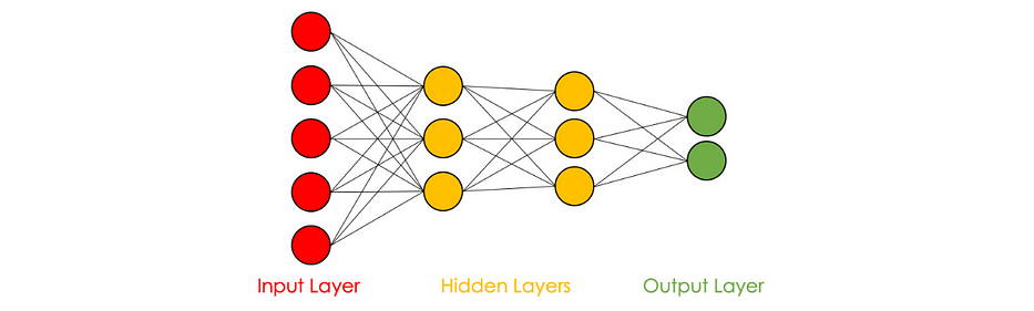
In general, neural networks better known as MLP, for ‘Multi Layers Perceptron’, is a type of direct formal neural network organized into several layers in which information flows from the input layer to the output layer only.

Each layer consists of a defined number of neurons, we distinguish :

- The input layer

- The hidden layers

- The output layer

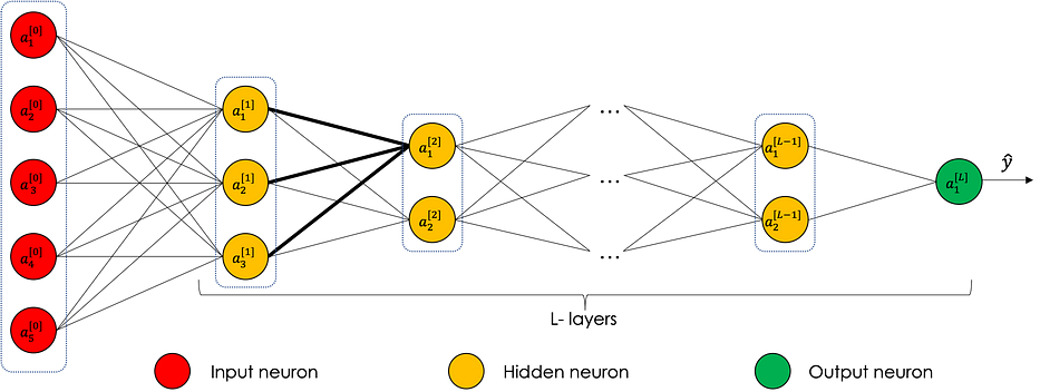
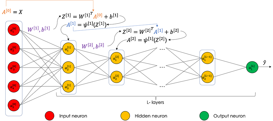
The following graph represents a neural network with 5 neurons at the input, 3 in the first hidden layer, 3 in the second hidden layer and 2 out.

Some variables in the hidden layers can be interpreted based on the input features: in the case of the house pricing and under the assumption that the first neuron of the first hidden layer pays more attention to the variables x_1​ et x_2​, it can be interpreted as the quantification of the family size of the house for instance.

DL as a supervised task

In most DL problems, we tend to predict an output y using a set of variables X, in this case, we suppose that for each row of the database X_i​ we have the corresponding prediction y_i​, thus the labeled data.

Applications: Real Estate, Speech Recognition, Image Classification …

The used data can be:

• Structured: explicit databases with features well defined
• Unstructured: Audio, Image, Text, …

Universal approximation theorem

Deep learning in real life is the approximation of a given function f. This approximation is possible and accurate thanks to the following theorem:

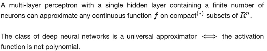
(*) In finite dimension, a set is said to be compact if it is closed and bounded. Visit this link for more details.
The main take-out of this algorithm is that deep learning allows solving any problem which can be mathematically expressed

Data Preprocessing

In any machine learning project in general, we divide our data into 3 sets:

- Train set: used to train the algorithm and construct batches

- Dev set: used to finetune the algorithm and evaluate bias and variance

- Test set: used to generalize the error/precision of the final algorithm

The following table sums up the repartition of the three sets according to the size of the data set m:

Standard deep learning algorithms require a large dataset where the number of samples is around lines. Now that the data is ready we will see in the next section the training algorithm.
Usually, before splitting the data, we also normalize the inputs, a step detailed later in this article.

‍

Learning algorithm

Learning in neural networks is the step of calculating the weights of the parameters associated with the various regressions throughout the network. In other words, we aim to find the best parameters that give the best prediction/approximation, starting from the input, of the real value.
For this, we define an objective function called the loss function and denoted J which quantifies the distance between the real and the predicted values on the overall training set.
We minimize J following two major steps:

- Forward Propagation: we propagate the data through the network either in entirely or in batches, and we calculate the loss function on this batch which is nothing but the sum of the errors committed at the predicted output for the different rows.

- Backpropagation: consists of calculating the gradients of the cost function with respect to the different parameters, then apply a descent algorithm to update them.

We iter the same process a number of times called epoch number. After defining the architecture, the learning algorithm is written as follows:

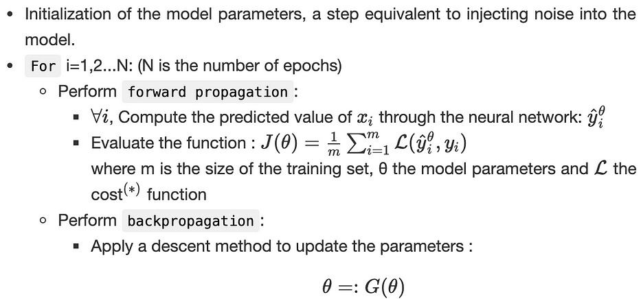
(∗) The cost function L evaluates the distances between the real and predicted value on a single point.

‍

Parameters’ initialization

The first step after defining the architecture of the neural network is parameter initialization. It is equivalent to injecting initial noise into the model’s weights.

• Zero initialization: one can think of initializing the parameters with 0’s everywhere i.e: W=0 and b=0

Using the forward propagation equations, we note that all the hidden units will be symmetric which penalizes the learning phase.

• Random initialization: it’s an alternative commonly used and consists of injecting random noise in the parameters. If the noise is too large, some activation functions might get saturated which might later affect the computation of the gradient.

Two of the most famous initialization methods are:

• Xavier's: it consists of filling the parameters with values randomly sampled from a centered variable following the normal distribution:

• Glorot's: the same approach with a different variance:

Forward and Backpropagation

Before diving into the algebra behind deep learning, we will first set the annotation which will be used in expliciting the equations of both the forward and the backpropagation.

Neural Network’s representation

The neural network is a sequence of regressions followed by an activation function. They both define what we call the forward propagation. and are the learned parameters at each layer. The backpropagation is also a sequence of algebraic operations carried out from the output towards the input.

Forward propagation

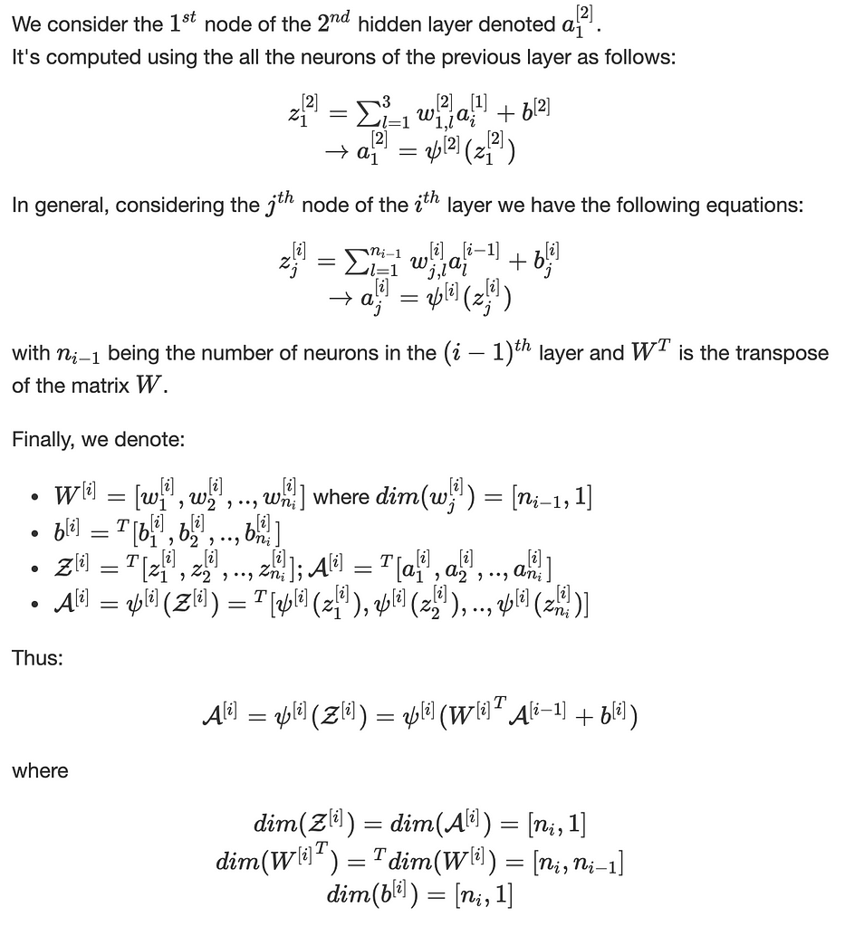
• Algebra through the network

Let us consider a neural network having L layers as follows:

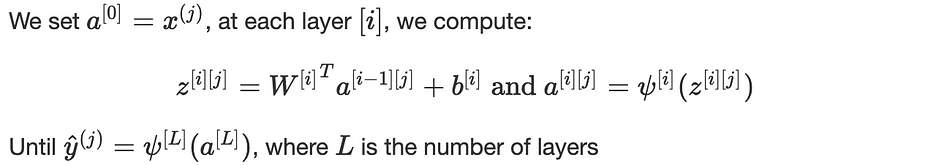
Algebra through the training set

Let us consider the prediction of the output of a single row data frame, through the neural network.

When dealing with a m-row data set, repeating these operations separately for each line is very costly.
We have, at each layer [i]:

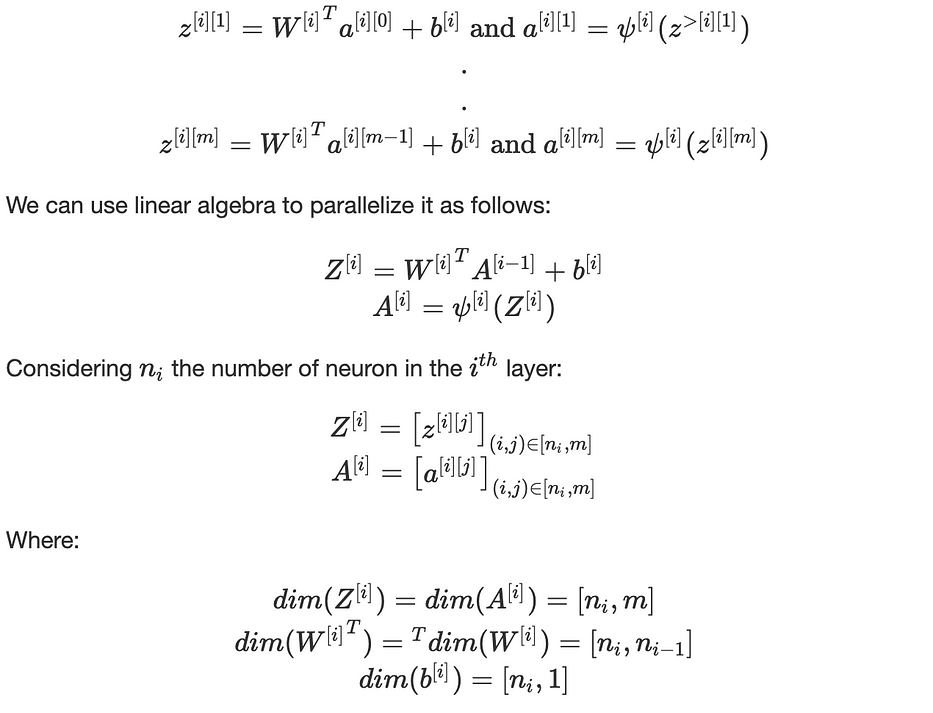
The parameter b_i uses broadcasting to repeat itself through the columns. This can be summarized in the following graph:

Backpropagation

The backpropagation is the second step of the learning, which consists of injecting the error committed in the prediction (forward) phase into the network and update its parameters to perform better on the next iteration.
Hence, the optimization of the function J, usually through a descent method.

Computational graph

Most of the descent methods require the computation of the gradient of the loss function denoted ∇J(θ).

In a neural network, the operation is carried out using a computational graph which decomposes the function J into several intermediate variables.

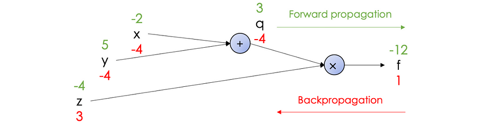
Let us consider the following function: f(x,y,z)=(x+y).z

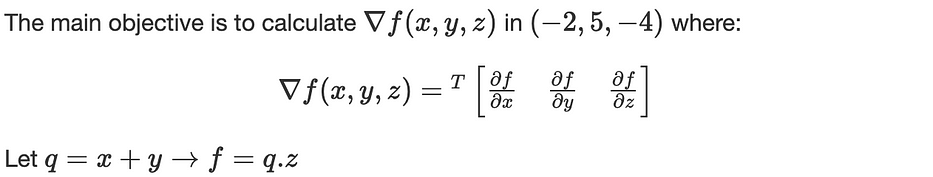
We carry out the computation using two passes:

• Forward propagation: computes the value of f from inputs to output: f(−2,5,−4)=−12
• Backpropagation: recursively apply chain-rule to compute gradients from output to inputs:

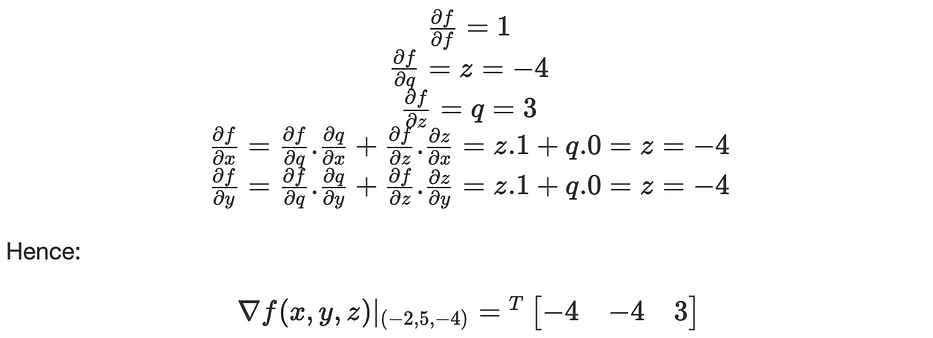
The derivatives can be resumed in the following computational graph:

Equations

Mathematically, we compute the gradients of the cost function J, w.r.t the architecture’s parameters W and b.

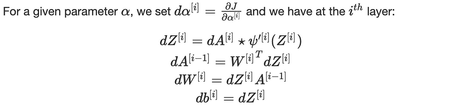
where (⋆) is the element-wise multiplication.
We recursively apply these equations for i=L, L−1,…,1

Gradient Checking

When carrying out the backpropagation, an additional checking is added to make sure that the algebraic computations are correct.

Algorithm:

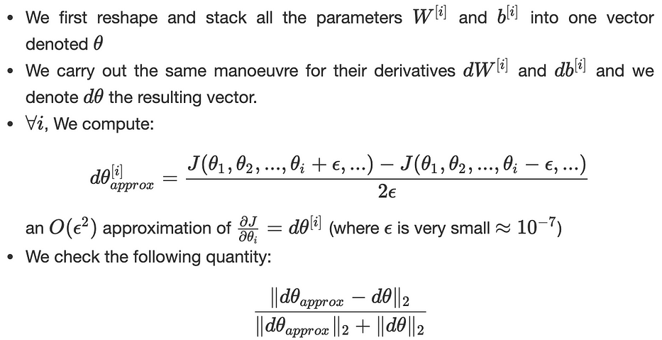
It should be close to the value of ϵ, an error is suspected when the value of the quantity is a thousand times higher than ϵ.

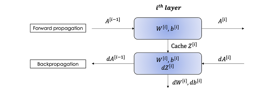
We can sum up the Forward and Backward propagation in the following block:

Parameters vs Hyperparameters

-Parameters, denoted θ, are the elements that we learn through the iterations and on which we apply backpropagation and update: W and b.

-Hyperparameters are all the other variables we define in our algorithm which can be tunned in order to improve the neural network:

• Learning rate α
• Number of iterations
• Choice of activation functions
• Number of layers L
• Number of units in each layer

‍

Activation functions

Activation functions are a kind of transfer functions that select the data propagated in the neural network. The underlying interpretation is to allow a neuron in the network to propagate learning data (if it is in a learning phase) only if it is sufficiently excited.

Here is a list of the most common functions:

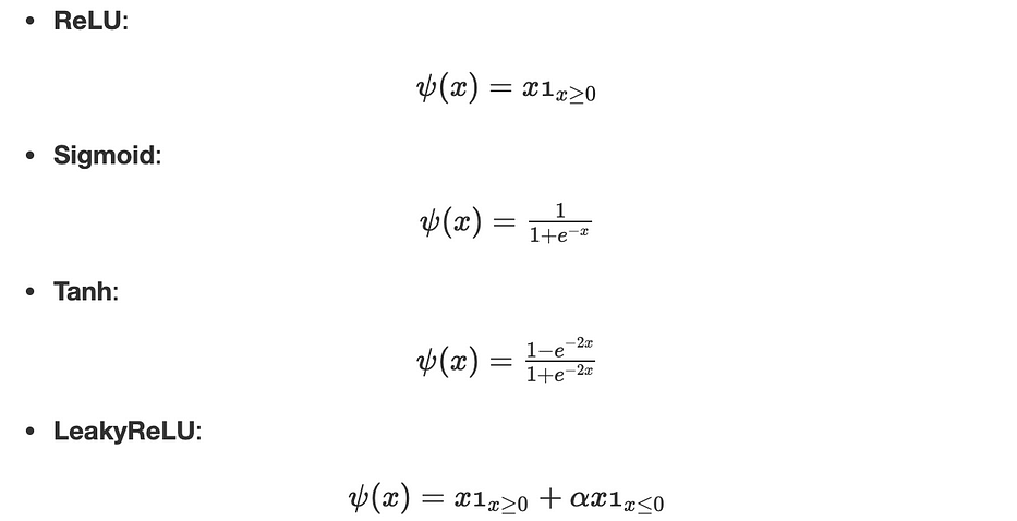
Remark: if the activation functions are all linear, the neural network is precisely equivalent to a simple linear regression

‍

Optimization algorithm

Risk

Let us consider a neural network denoted by f. The real objective to optimize is defined as the expected loss over all the corpora:

Where X is an element from a continuous space of observables to which correspond a target Y and p(X,Y) being the marginal probability of observing the couple (X,Y).

Empirical risk

Since we can not have all the corpora and hence we ignore the distribution, we restrict the estimation of the risk on a certain dataset well representative of the overall corpora and consider all the cases equiprobable.
In this case: we set m to be the size of the representative corpora, we get :∫=∑ and p(X,Y)=1/m. Hence, we iteratively optimize the loss function defined as follows:

Plus we can assert that:

There exist many techniques and algorithms, mainly based on gradient descent, which carries out the optimization. In the sections below, we will go through the most famous ones. It is important to note that these algorithms might get stuck in local minima and nothing assures reaching the global one.

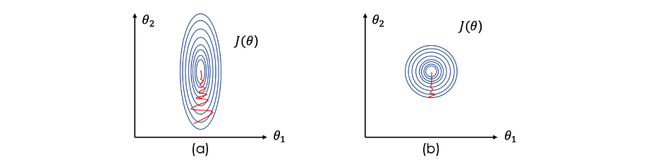
Normalizing inputs

Before optimizing the loss function, we need to normalize the inputs in order to speed up the learning. In this case, J(θ) becomes tighter and more symmetric which helps gradient descent to find the minimum faster and thus in fewer iterations.
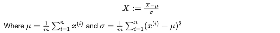
Standard data is the commonly used approach which consists of subtracting the mean of the variables and dividing by their standard deviation. Considering, the following image illustrates the effect of normalizing the input on the contour lines of -standard data on the right-:

Let X be a variable in our database, we set:

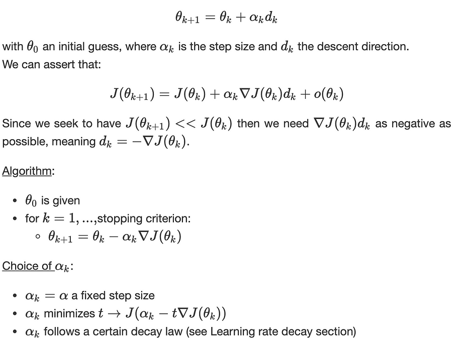
Gradient descent

In general, we tend to construct a convex and differentiable function J where any local minima is a global one. Mathematically speaking finding the global minimum of a convex function is equivalent to solving the equation ∇J(θ)=0, we denote θ⋆ its solution.
Most of the used algorithms are of the kind:

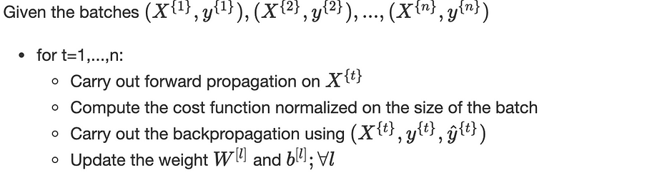
Mini-batch gradient descent

This technique consists of dividing the training set to batches:

Choice of the mini-batch size:

• A small number of rows ∼2000 lines
• Typical size: the power of 2 which is good for memory
• Mini-batch should fit in CPU/GPU memory

Remark: in the case where there is only one data line in the batch, the algorithm is called stochastic gradient descent

Gradient descent with momentum

A variant of gradient descent which includes the notion of momentum, the algorithm is as follows:

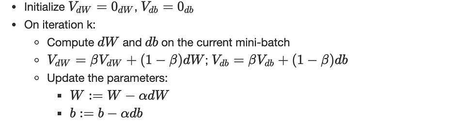
(α,β) are hyperparameters.
Since dθ is calculated on a mini-batch, the resulting gradient ∇J is very noisy, this exponentially weighted averages included by the momentum give a better estimation of derivatives.

RMSprop

Root Mean Square prop is very similar to gradient descent with momentum, the only difference is that it includes the second-order momentum instead of the first-order one, plus a slight change on the parameters’ update:

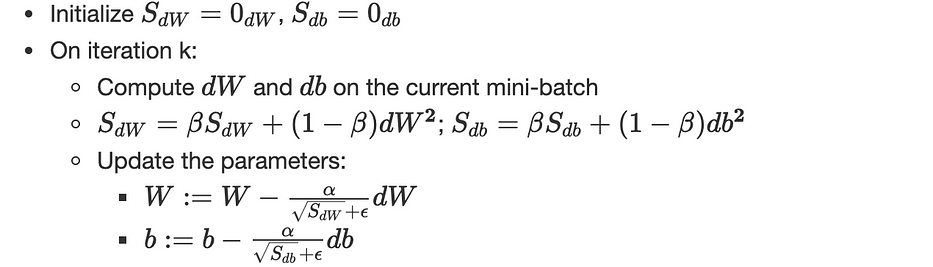
(α,β) are hyperparameters and ϵ assures numerical stability (≈10−8)

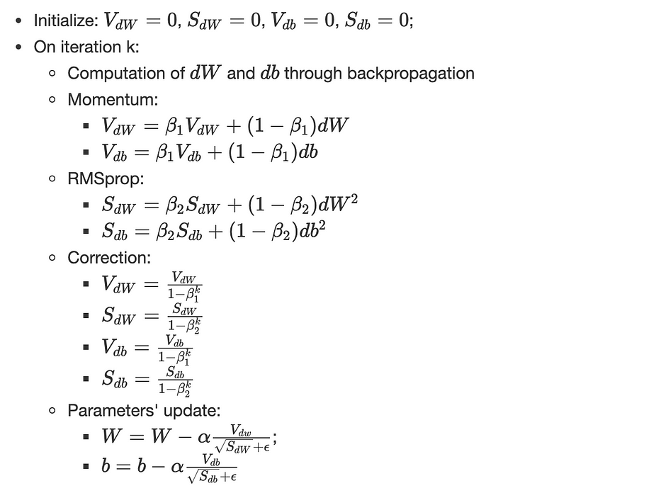
Adam

Adam is an adaptive learning rate optimization algorithm designed specifically for training deep neural networks. Adam can be seen as a combination of RMSprop and gradient descent with momentum.
It uses square gradients to set the learning rate at scale as RMSprop and takes advantage of momentum by using the moving average of the gradient instead of the gradient itself as the gradient descends with momentum.
The main idea is to avoid oscillations during optimization by accelerating the descent in the right direction.
The algorithm of Adam optimizer is the following:

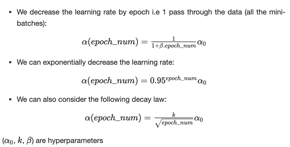
Learning rate decay

The main objective of the learning rate decay is to slowly reduce the learning rate over time/iterations. It finds justification in the fact that we afford to take big steps at the beginning of the learning but when approaching the global minimum, we slow down and thus decrease the learning rate.
There exist many learning rate decay laws, here are some of the most common:

Regularization

Variance/bias

When training a neural network, it might suffer from:

• High bias: or underfitting, where the network fails to find the path in the data, in this case, J_train​ is very high the same as J_dev​. Mathematically speaking, when performing cross-validation; the mean of J on all the considered folds is high.
• High variance or overfitting, the model fits perfectly on the training data but fails to generalize on unseen data, in this case, J_train​ is very low and J_dev​ is relatively high. Mathematically speaking, when performing cross-validation; the variance of J on all the considered folds is high.

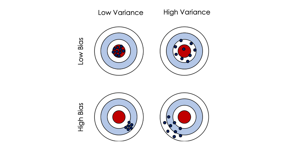
Let’s consider the dartboard game, where hitting the red target is the best-case scenario. Having a low bias (first line) means that on average we are close to the goal. In case, of a low variance, the hits are all concentrated around the target (the variance of the hits’ distribution is low). When the variance is high, under the assumption of a low bias, the hits are spread out but still around the red circle.
Vice-versa, we can define the high bias with a low/high variance.

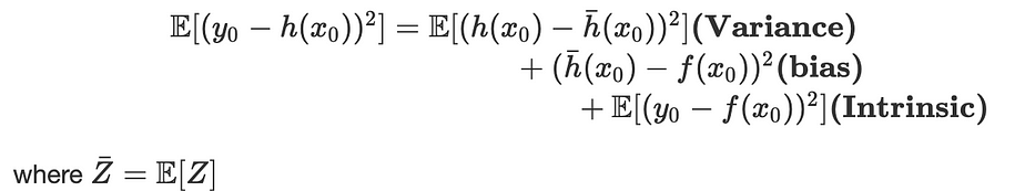
Mathematically speaking, let f be a true regression function: y=f(x)+ϵ where: ϵ~N(0,σ²)
We fit a hypothesis h(x)=Wx+b with MSE and consider x_0​ be a new data point, y_0​=f(x_0​)+ϵ: the expected error can be defined by:

A trade-off must be found between variance and bias to find the optimum complexity of the model either by using the AIC criteria or using cross-validation.
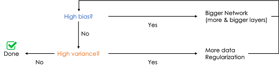
Here is a simple schema to follow to solve bias/variance issues:

L1 — L2 regularization

Regularization is an optimization technique that prevents overfitting.
It consists of adding a term in the objective function to minimize as follows:

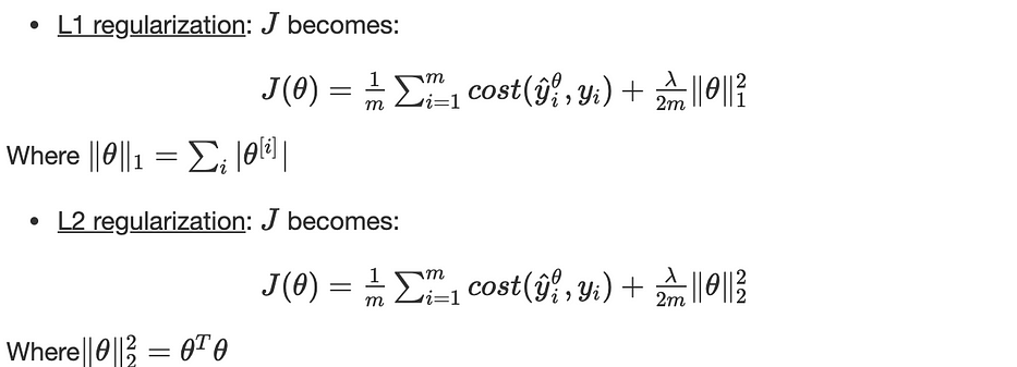
λ is the hyperparameter of the regularization.

Backpropagation and regularization
The update of the parameters during backpropagation depends on the gradient ∇J, to which is added a new regularization term. In L2 regularization, it becomes as follows:

Considering λ>>1, minimizing the cost function leads to weak values of parameters because of the term (λ/2m)​∥θ∥ which simplifies the network and makes more consistent, hence less exposed to overfitting.

Dropout regularization

Roughly speaking, the main idea is to sample a uniform random variable, for each layer for each node, and have p chance of keeping the node and 1−p of removing it which diminishes the network.
The main intuition of dropout is based on the idea that the network shouldn't rely on a specific feature but should instead spread out the weights!
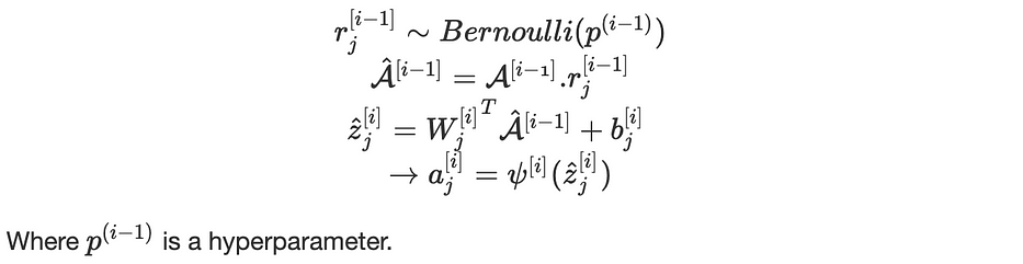
Mathematically speaking, when dropout is off and considering the j th node of the i th layer, we have the following equations:

When dropout is on, the equations become as follows:

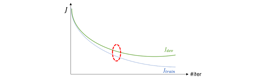
Early stopping

This technique is quite simple and consists of stopping the iteration around the area when J_train​ and J_dev​ start separating:

Gradient problems

The computation of gradients suffers from two major problems: gradient vanishing and gradient exploding.
To illustrate both of the situations, let’s consider a neural network where all the activation functions ψ[i] are linear and:

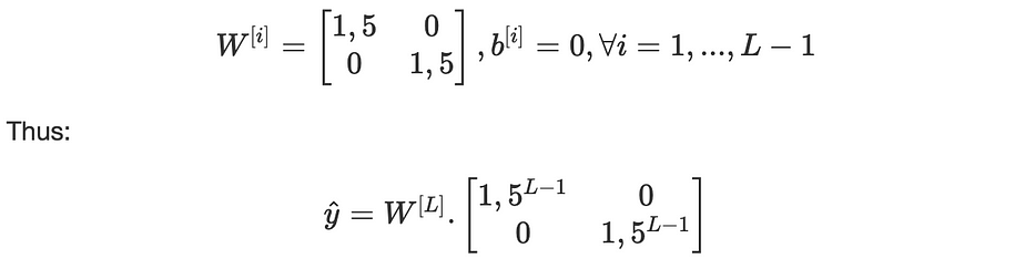
We note that 1,5^(L−1) will explode exponentially as a function of the depth L. If we use 0.5 instead of 1,5 then 0,5^(L-1) will vanish exponentially as well.
The same issue occurs with gradients.

‍

Conclusion

As a data scientist, it is very important to be aware of the mathematics turning in the background of the neural networks. This allows better understanding and faster debugging.

Do not hesitate to check my previous article dealing with:

• Convolutional Neural Networks’ mathematics
• Object detection & Face recognition algorithms
• Recurrent Neural Networks

Happy Machine Learning!

‍

References

• Deep Learning Specialization, Coursera, Andrew Ng
• Optimization course, Mines Nancy, Antoine Henrot
• Machine Learning, Loria, Christophe Cerisara