Computer vision is a subfield of deep learning which deals with images on all scales. It allows the computer to process and understand the content of a large number of pictures through an automatic process.
The main architecture behind Computer vision is the convolutional neural network which is a derivative of feedforward neural networks. Its applications are very various such as image classification, object detection, neural style transfer, face identification,… If you have no background on deep learning in general, I recommend you to first read my  about feedforward neural networks.

NB: Since Medium does not support LaTeX, the mathematical expressions are inserted as images. Hence, I advise you to turn the dark mode off for a better reading experience.

The summary is as follows:

1. Filter processing
2. Definitions
3. Foundations
4. Training the CNN
5. Common architectures

‍

Filter processing

The first processing of images was based on filters that allowed, for instance, to get the edges of an object in an image using the combination of vertical-edge and horizontal-edge filters.
Mathematically speaking, the vertical edge filter, VEF, if defined as follows:

Where HEF stands for the horizontal edge filter.

For the sake of simplicity, we consider grayscale 6x6 image A, a 2D matrix where the value of each element represents the amount of light in the corresponding pixel.
In order to extract the vertical edges from this image, we carry out a convolutional product (⋆) which is basically the sum of the elementwise product in each block:

We carry out the elementwise multiplication on the first 3x3 block of the image then we consider the following block on the right and do the same thing until we have covered all the potential blocks.

We can sum up the following process in:

Given this example, we can think of using the same process for any objective where the filter is learned by neural network as follows:

The main intuition is to set a neural network that takes the image as an input and outputs a defined target. The parameters are learned using backpropagation.

‍

Definition

A convolutional neural network is a serie of convolutional and pooling layers which allow extracting the main features from the images responding the best to the final objective.

In the following section, we will detail each brick along with its mathematical equations.

Convolution product

Before we explicitly define the convolution product, we will first start by defining some basic operations such as the padding and the stride.

Padding

As we have seen in the convolutional product using the vertical-edge filter, the pixels on the corner of the image (2D matrix) are less used than the pixels in the middle of the picture which means that the information from the edges is thrown away.
To solve this problem, we often add padding around the image in order to take the pixels on the edges into account. In convention, we padde with zeros and denote with p the padding parameter which represents the number of elements added on each of the four sides of the image.
The following picture illustrates the padding of a grayscale image (2D matrix) where p=1:

Stride

The stride is the step taken in the convolutional product. A large stride allows to shrink the size of the output and vice-versa. We denote s the stride parameter.
The following image illustrates a convolutional product (sum of element-wise element per block) with s=1:

Convolution

Once we have defined the stride and the padding we can define the convolution product between a tensor and a filter.
After previously defining the convolution product on a 2D matrix which is the sum of the element-wise product, we can now formally define the convolution product on a volume.
An image, in general, can be mathematically represented as a tensor with the following dimensions:

In the case of an RGB image, for instance, n_C=3, we have, Red, Green and Blue. In convention, we consider the filter K to be squared and to have an odd dimension denoted f, which allows each pixel to be centered in the filter and thus consider all the elements around it.
When operating the convolutional product, the filter/kernel K must have the same number of channels as the image, this way we apply a different filter to each channel. Thus the dimension of the filter is as follows:

The convolutional product between the image and the filter is a 2D matrix where each element is the sum of the elementwise multiplication of the cube (filter) and the subcube of the given image as illustrated below:

Mathematically speaking, for a given image and filter we have:

Keeping the same notations as before, we have:

Pooling

It is the step of downsampling the image’s features through summing up the information. The operation is carried out through each channel and thus it only affects the dimensions (n_H, n_W)and keeps n_C intact.
Given an image, we slide a filter, with no parameters to learn, following a certain stride, and we apply a function on the selected elements. We have:

In convention, we consider a squared filter with size f and we usually set f=2 and consider s=2.

We often apply:

• Average pooling: we average on the elements present on the filter
• Max pooling: given all the elements in the filter, we return the maximum

Bellow, an illustration of an average pooling:

‍

Foundations

In this section, we will combine all the operations defined above to construct a convolutional neural network, layer per layer.

One layer of a CNN

Each layer of the convolutional neural network can either be:

• Convolutional layer -CONV- followed with an activation function
• Pooling layer -POOL- as detailed above
• Fully connected layer -FC- a layer which is basically similar to one from a feedforward neural network,

You can have more details on the activations functions and the fully connected layer in my previous post.

• Convolutional layer

As we have seen before, at the convolutional layer, we apply convolutional products, using many filters this time, on the input followed by an activation function ψ.

We can sum up the convolutional layer in the following graph:

• Pooling layer

As mentioned before, the pooling layer aims at downsampling the features of the input without impacting the number of the channels.
We consider the following notation:

We can assert that:

The pooling layer has no parameters to learn.

We sum up the previous operations in the following illustration:

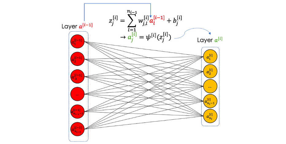
• Fully connected layer

A fully connected layer is a finite number of neurons which takes in input a vector and returns another one.

We sum up the fully connected layer in the following illustration:

For more details, you can visit my previous article on feedforward neural networks.

CNN in Overall

In general, a convolutional neural network is a serie of all the operations described above as follows:

After repeating a serie of convolutions followed by activation functions, we apply a pooling and repeat this process a certain number of time. These operations allow to extract features from the image that will be fed to a neural network described by the fully connected layers which are regularly followed by activation functions as well.
The main idea is to decrease n_H & n_W and increase n_C when going deeper through the network.
In 3D, a convolutional neural network has the following shape:

Why do CNN work efficiently?

Convolutional neural networks enable the state of the art results in image processing for two main reasons:

• Parameter sharing: a feature detector in the convolutional layer which is useful in one part of the image, might be useful in other ones
• Sparsity of connections: in each layer, each output value depends only on a small number of inputs

‍

Training the CNN

Convolutional neural networks are trained on a set of labeled images. Starting from a given image, we propagate it through the different layers of the CNN and return the sought output.
In this chapter, we will go through the learning algorithm along with the different techniques used in the data augmentation.

Data preprocessing

Data augmentation is the step of increasing the number of images in a given dataset. There are many techniques used in data augmentation such as:

• Crooping
• Rotation
• Flipping
• Noise injection
• Color space transformation

It enables better learning due to the bigger size of the training set and allows the algorithm to learn from different conditions of the object in question.
Once the dataset is ready, we split it into three parts like any machine learning project:

• Train set: used to train the algorithm and construct batches
• Dev set: used to finetune the algorithm and evaluate bias and variance
• Test set: used to generalize the error/precision of the final algorithm

Learning algorithm

Convolutional neural networks are a special kind of neural networks specialized in images. Learning in neural networks, in general, is the step of calculating the weights of the parameters defined above in several layers.
In other words, we aim to find the best parameters that give the best prediction/approximation, starting from the input image, of the real value.
For this, we define an objective function called the loss function and denoted J which quantifies the distance between the real and the predicted values on the overall training set.
We minimize J following two major steps:

• Forward Propagation: we propagate the data through the network either in entirely or in batches, and we calculate the loss function on this batch which is nothing but the sum of the errors committed at the predicted output for the different rows.
• Backpropagation: consists of calculating the gradients of the cost function with respect to the different parameters, then apply a descent algorithm to update them.

We iter the same process a number of times called epoch number. After defining the architecture, the learning algorithm is written as follows:

(*) The cost function evaluates the distances between the real and predicted value on a single point.

For more details, you can visit my previous article‍ on feedforward neural networks.

Common architectures

Resnet

A Resnet, short cut or a skip connection is a convolutional layer which takes into account the layer n-2 at the layer n . The intuition comes from the fact that when neural networks get very deep, the accuracy at the output becomes very stable and does not increase. Injecting residuals from the previous layer help solve this problem.
Let’s consider a residual block, when the skip connection is off, we have the following equations:

We can sum up the residual block in the following illustration:

Inception Networks

When designing a convolutional neural network, we often have to choose the type of the layer: CONV, POOL or FC. The inception layer does them all. The result of all the operations is then concatenated in a single block which will be the input of the next layer as follows:

It is important to note that the inception layer raises the problem of computational cost. For information, the name inception comes from the movie!

‍

Conclusion

In the first part of this article, we have seen the fundamentals of CNN from convolutional products, pooling/fully connected layers to the training algorithm.

In the second part, we will discuss some of the most famous architectures used in image processing.

Do not hesitate to check my previous article dealing with:

• Deep Learning’s mathematics
• Object detection & Face recognition algorithms
• Recurrent Neural Networks

‍

References

• Deep Learning Specialization, Coursera, Andrew Ng
• Machine Learning, Loria, Christophe Cerisara